Peak Energy Prediction

Introduction

With global energy usage rapidly increasing and the switch to renewable energy being slow and often ineffective, fluctuations in energy supply and demand have been known to put extreme strain on energy grids. In Western Australia, the South-West Interconnected System (SWIS) is no different. Energy suppliers in WA have a reserve capacity requirement to ensure peak demand can be met throughout the year, with the suppliers charging a premium price to users on the four peak energy demand days of the hot season (December 1 to March 31). A company can therefore mitigate costs if they know when these four peak demand days will be and lower their usage on those days.

The objective of our project was to forecast energy demand in WA using machine learning algorithms with the primary goal of forecasting the four peak energy use days. We trained these models on a dataset of hourly energy demand and weather data over the last 15 years. From early data exploration, it was understood that energy demand was time dependent. Accordingly, we prioritised models that captured this property and performed feature engineering to encapsulate the cyclical nature of temperature and weather across days and seasons

Data Exploration

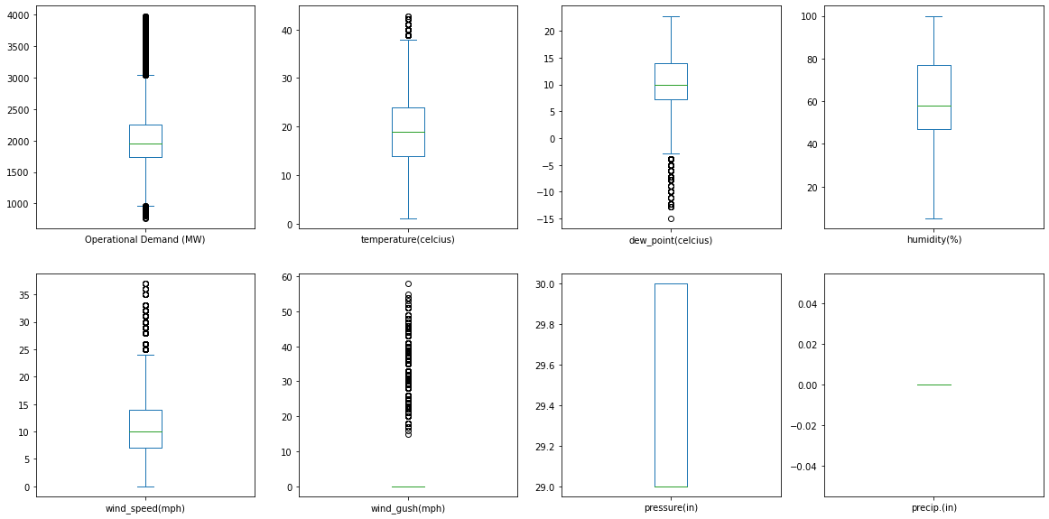
On the initial data exploration, it was also seen that the hourly temperature and the dew point exhibited a sinusoidal pattern (figure 1 & 2). The data extracted from the weather underground consisted of various other features like wind gust and precipitation which were proven to be insignificant on the initial exploration (figure 3). As a result, these were removed from the dataset. The data exploration aided in understanding a pattern which already existed in the data which was helpful in inferring the reason behind a peak in the energy consumption. Since the climatic features are adverse during this time of the year, the consumers are forced to depend on the electronic devices to keep themselves unaffected by the weather.

Approach

Initially the utilisation of some classical statistical approaches coupled with regression models were used for knowledge discovery to decide which advanced models should be considered. As such, a Convolutional Neural Network, a gradient boosting model through XGBoost, and a Decision Tree were adopted to attempt to forecast energy demand. With energy demand forecasted, we could then compare this to a baseline from previous years to determine the probability that each forecasted day would exceed that baseline and become one of the four peak energy usage days. This also allowed us to introduce an aspect of responsible data science, by which the decision to lower energy usage is not made by the model, but rather made with the model's predictions used to support that decision.

Feature Engineering

Under the assumption that the consumption prediction is not solely based on the climatic data, new features like 'hour of day', 'day of week', 'quarter of year', 'month of year', 'year', 'day of year', 'day of month' and 'week of year' were added as features in addition to the climatic features like 'hourly temp', 'dew point', 'humidity', 'wind speed', 'pressure' were used for the modelling. As it says that the history always repeats, the time seems to play a very significant role in predicting the independent variable.

XGBoost

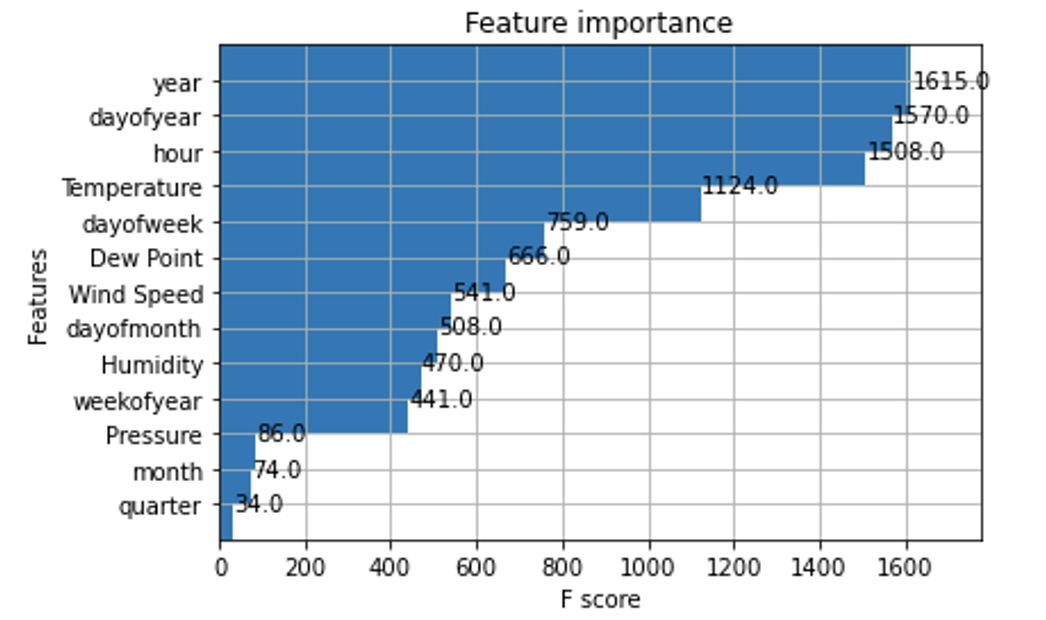
Using the XGBRegressor from the xgboost library a model was derived using the above-mentioned features. By feeding in 13 input features, an output variable was fitted and predicted later. From the model, the year and the day of year had the most significance as assumed earlier. Quarter of the year had the least importance (figure 4). The temperature out of all the climatic features has the most significance. It is self-explanatory that with the increase in temperature, the consumers are forced to use the air conditioning and vice versa.

The XGBoost technique offers several benefits in terms of model prediction, including the lack of data pre-processing, a quick operation speed, complete feature extraction, a strong fitting effect, and high prediction accuracy. We, therefore, chose an XGBoost model to compare its effectiveness with ARIMA, given its ability to outperform ARIMA on multiple occasions. Given that the model does not operate as a time-series model, it is more interpretable and more capable of operating on isolated days without requiring sequential input as with the other models.

The model was then used to predict the consumption of the past summer (2021-22) and the results were quite promising. The predicted values were then plotted against the actual values (figure 5) to examine the reproduction. On evaluating the result, the root mean square error (RSME) was obtained to be 215.26 which was a lower value. The MAPE value was also calculated to be 7.2% which also gave the model a fair upper hand over the base model.

Forecasting

The weather forecast were obtained using weather api. The api fetches the weather forecast data starting from the next hour for the next 14 days. Using the data, initially a forecast for the next 14 days was made to obtain the results (figure 6).

Later, the weather forecast for the next 48 hours were obtained with the top 2 peaks of the day plotted (figure 7).

Future Improvements

A future improvement for this model could be exploring the Regression/Residuals approach adopted by the SARIMA model, but instead couple it with more interpretable models. This would make each prediction based on a simple, explainable multi-linear regression, which as mentioned above can be incredibly successful in various modelling situations.

Another potential improvement in the models could be made by including a solar irradiation feature. High irradiation days will cause a decrease in energy usage when solar power is significant enough. Unfortunately, no such data was publicly available. This could be investigated at a later date with appropriate funding.